Expand broom::tidy() Outputs for Categorical Parameter Estimates

Create additional columns in a tidy model output (such as broom::tidy.lm()) to allow for easier control when plotting categorical parameter estimates.

Usage

tidy_categorical(
  d = NULL,
  m = NULL,
  include_reference = TRUE,
  reference_label = "Baseline Category",
  non_reference_label = paste0("Non-", reference_label),
  exponentiate = FALSE,
  n_level = FALSE
)

Arguments

d: A data frame tibble::tibble() output from broom::tidy.lm(); with one row for each term in the regression, including column term
m: A model object, created using a function such as lm()
include_reference: Logical indicating to include additional rows in output for reference categories, obtained from dummy.coef(). Defaults to TRUE
reference_label: Character string. When used will create an additional column in output with labels to indicate if terms correspond to reference categories.
non_reference_label: Character string. When reference_label is used will be in output to indicate if terms not corresponding to reference categories.
exponentiate: Logical indicating whether or not the results in broom::tidy.lm() are exponentiated. Defaults to FALSE.
n_level: Logical indicating whether or not to include a column n_level for the number of observations per category. Defaults to FALSE.

Value

Expanded tibble::tibble() from the version passed to d including additional columns:

variable: The name of the variable that the regression term belongs to.
level: The level of the categorical variable that the regression term belongs to. Will be an the term name for numeric variables.
effect: The type of term (main or interaction)
reference: The type of term (reference or non-reference) with label passed from reference_label. If reference_label is set NULL will not be created.
n_level: The the number of observations per category. If n_level is set NULL (default) will not be created.

In addition, extra rows will be added, if include_reference is set to FALSE for the reference categories, obtained from dummy.coef()

Author

Guy J. Abel

Examples

# strip ordering in factors (currently ordered factor not supported)
library(dplyr)
#> 
#> Attaching package: ‘dplyr’
#> The following objects are masked from ‘package:stats’:
#> 
#>     filter, lag
#> The following objects are masked from ‘package:base’:
#> 
#>     intersect, setdiff, setequal, union
library(broom)

m0 <- esoph %>%
  mutate_if(is.factor, ~factor(., ordered = FALSE)) %>%
  glm(cbind(ncases, ncontrols) ~ agegp + tobgp * alcgp, data = .,
        family = binomial())
# tidy
tidy(m0)
#> # A tibble: 21 × 5
#>    term        estimate std.error statistic  p.value
#>    <chr>          <dbl>     <dbl>     <dbl>    <dbl>
#>  1 (Intercept)    -7.27     1.11      -6.57 5.15e-11
#>  2 agegp35-44      1.90     1.11       1.72 8.62e- 2
#>  3 agegp45-54      3.70     1.06       3.48 5.06e- 4
#>  4 agegp55-64      4.25     1.06       4.00 6.25e- 5
#>  5 agegp65-74      4.81     1.07       4.50 6.83e- 6
#>  6 agegp75+        4.79     1.12       4.26 2.00e- 5
#>  7 tobgp10-19      1.30     0.491      2.65 8.16e- 3
#>  8 tobgp20-29      1.41     0.606      2.33 1.98e- 2
#>  9 tobgp30+        2.16     0.644      3.35 8.06e- 4
#> 10 alcgp40-79      2.02     0.403      5.02 5.18e- 7
#> # ℹ 11 more rows

# add further columns to tidy output to help manage categorical variables
m0 %>%
 tidy() %>%
 tidy_categorical(m = m0, include_reference = FALSE)
#> # A tibble: 21 × 8
#>    term        estimate std.error statistic  p.value variable    level    effect
#>    <chr>          <dbl>     <dbl>     <dbl>    <dbl> <chr>       <fct>    <chr> 
#>  1 (Intercept)    -7.27     1.11      -6.57 5.15e-11 (Intercept) (Interc… main  
#>  2 agegp35-44      1.90     1.11       1.72 8.62e- 2 agegp       35-44    main  
#>  3 agegp45-54      3.70     1.06       3.48 5.06e- 4 agegp       45-54    main  
#>  4 agegp55-64      4.25     1.06       4.00 6.25e- 5 agegp       55-64    main  
#>  5 agegp65-74      4.81     1.07       4.50 6.83e- 6 agegp       65-74    main  
#>  6 agegp75+        4.79     1.12       4.26 2.00e- 5 agegp       75+      main  
#>  7 tobgp10-19      1.30     0.491      2.65 8.16e- 3 tobgp       10-19    main  
#>  8 tobgp20-29      1.41     0.606      2.33 1.98e- 2 tobgp       20-29    main  
#>  9 tobgp30+        2.16     0.644      3.35 8.06e- 4 tobgp       30+      main  
#> 10 alcgp40-79      2.02     0.403      5.02 5.18e- 7 alcgp       40-79    main  
#> # ℹ 11 more rows

# include reference categories and column to indicate the additional terms
m0 %>%
 tidy() %>%
 tidy_categorical(m = m0)
#> # A tibble: 31 × 9
#>    term    estimate std.error statistic  p.value variable level effect reference
#>    <chr>      <dbl>     <dbl>     <dbl>    <dbl> <chr>    <fct> <chr>  <chr>    
#>  1 (Inter…    -7.27     1.11      -6.57 5.15e-11 (Interc… (Int… main   Non-Base…
#>  2 NA          0        0          0    0        agegp    25-34 main   Baseline…
#>  3 agegp3…     1.90     1.11       1.72 8.62e- 2 agegp    35-44 main   Non-Base…
#>  4 agegp4…     3.70     1.06       3.48 5.06e- 4 agegp    45-54 main   Non-Base…
#>  5 agegp5…     4.25     1.06       4.00 6.25e- 5 agegp    55-64 main   Non-Base…
#>  6 agegp6…     4.81     1.07       4.50 6.83e- 6 agegp    65-74 main   Non-Base…
#>  7 agegp7…     4.79     1.12       4.26 2.00e- 5 agegp    75+   main   Non-Base…
#>  8 NA          0        0          0    0        tobgp    0-9g… main   Baseline…
#>  9 tobgp1…     1.30     0.491      2.65 8.16e- 3 tobgp    10-19 main   Non-Base…
#> 10 tobgp2…     1.41     0.606      2.33 1.98e- 2 tobgp    20-29 main   Non-Base…
#> # ℹ 21 more rows

# coefficient plots
d0 <- m0 %>%
  tidy(conf.int = TRUE) %>%
  tidy_categorical(m = m0) %>%
  # drop the intercept term
  slice(-1)
d0
#> # A tibble: 30 × 11
#>    term   estimate std.error statistic p.value conf.low conf.high variable level
#>    <chr>     <dbl>     <dbl>     <dbl>   <dbl>    <dbl>     <dbl> <chr>    <fct>
#>  1 NA         0        0          0    0          0          0    agegp    25-34
#>  2 agegp…     1.90     1.11       1.72 8.62e-2    0.105      4.87 agegp    35-44
#>  3 agegp…     3.70     1.06       3.48 5.06e-4    2.04       6.63 agegp    45-54
#>  4 agegp…     4.25     1.06       4.00 6.25e-5    2.60       7.17 agegp    55-64
#>  5 agegp…     4.81     1.07       4.50 6.83e-6    3.14       7.75 agegp    65-74
#>  6 agegp…     4.79     1.12       4.26 2.00e-5    2.96       7.78 agegp    75+  
#>  7 NA         0        0          0    0          0          0    tobgp    0-9g…
#>  8 tobgp…     1.30     0.491      2.65 8.16e-3    0.331      2.28 tobgp    10-19
#>  9 tobgp…     1.41     0.606      2.33 1.98e-2    0.154      2.58 tobgp    20-29
#> 10 tobgp…     2.16     0.644      3.35 8.06e-4    0.837      3.40 tobgp    30+  
#> # ℹ 20 more rows
#> # ℹ 2 more variables: effect <chr>, reference <chr>

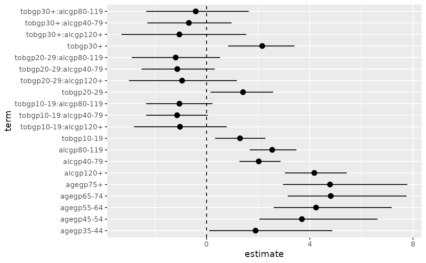
# typical coefficient plot
library(ggplot2)
library(tidyr)
ggplot(data = d0 %>% drop_na(),
       mapping = aes(x = term, y = estimate,
                     ymin = conf.low, ymax = conf.high)) +
  coord_flip() +
  geom_hline(yintercept = 0, linetype = "dashed") +
  geom_pointrange()


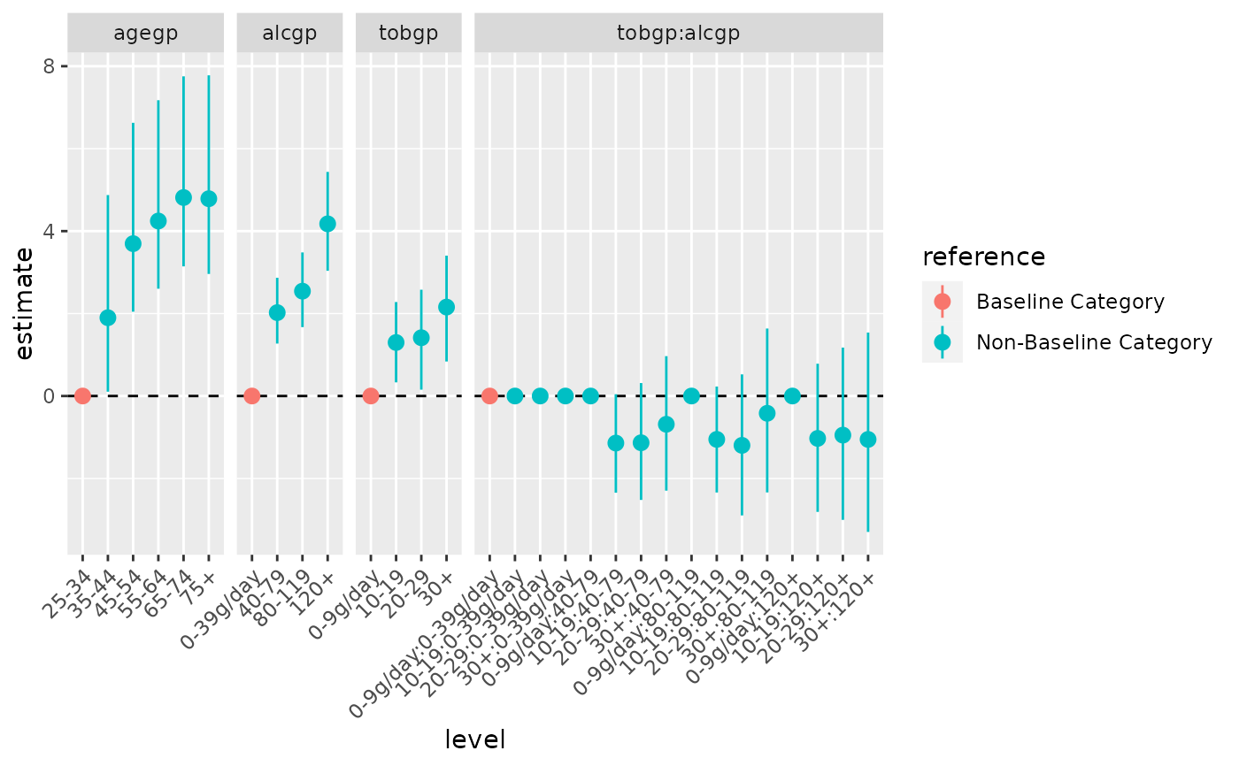
# enhanced coefficient plot using additional columns from tidy_categorical and ggforce::facet_row()
library(ggforce)
ggplot(data = d0,
       mapping = aes(x = level, colour = reference,
                     y = estimate, ymin = conf.low, ymax = conf.high)) +
  facet_row(facets = vars(variable), scales = "free_x", space = "free") +
  geom_hline(yintercept = 0, linetype = "dashed") +
  geom_pointrange() +
  theme(axis.text.x = element_text(angle = 45, hjust = 1))