tidycat

Introduction

The tidycat package includes the tidy_categorical() function to expand broom::tidy() outputs for categorical parameter estimates.

See the pkgdown site for full details.

Installation

You can install the released version of tidycat from CRAN with:

install.packages("tidycat")

And the development version from GitHub with:

# install.packages("devtools")
devtools::install_github("guyabel/tidycat")

Limitations

The tidy_categorical() function will probably not work as expected for non-default contrasts such as contr.helmert() and when one or more model parameters are rank deficient. It also only supports a limited range of models; lm() or glm() should be fine. For more complex cases, or an alternative method do create great coefficient plots, see the ggcoef_model() function in the GGally package, which went through a major upgrade around the same time as I developed tidycat.

Documentation

For full documentation, see the package vignette: The tidycat package: expand broom::tidy() output for categorical parameter estimates

Hello World

The tidy() function in the broom package takes the messy output of built-in functions in R, such as lm(), and turns them into tidy data frames.

library(dplyr)
library(broom)

m1 <- mtcars %>%
  mutate(transmission = recode_factor(am, `0` = "automatic", `1` = "manual")) %>%
  lm(mpg ~ as.factor(cyl) + transmission + wt *  as.factor(cyl), data = .)

tidy(m1)
#> # A tibble: 7 x 5
#>   term               estimate std.error statistic       p.value
#>   <chr>                 <dbl>     <dbl>     <dbl>         <dbl>
#> 1 (Intercept)          41.5        4.54     9.14  0.00000000190
#> 2 as.factor(cyl)6      -8.66      10.4     -0.836 0.411        
#> 3 as.factor(cyl)8     -16.9        5.27    -3.20  0.00374      
#> 4 transmissionmanual   -0.902      1.51    -0.595 0.557        
#> 5 wt                   -6.19       1.65    -3.75  0.000937     
#> 6 as.factor(cyl)6:wt    2.12       3.40     0.625 0.538        
#> 7 as.factor(cyl)8:wt    3.84       1.77     2.17  0.0399

The tidy_categorical() function adds

• further columns (variable, level and effect) to the broom::tidy() output to help manage categorical variables
• further rows for reference category terms and a column to indicate their location (reference) when setting include_reference = TRUE (default)

It requires two inputs

• a data frame d of parameter estimates from a model from broom::tidy()
• the corresponding model object m passed to broom::tidy()

For example:

library(tidycat)
d1 <- m1 %>%
  tidy(conf.int = TRUE) %>%
  tidy_categorical(m = m1)
d1 %>%
  select(-(3:5))
#> # A tibble: 10 x 8
#>    term               estimate conf.low conf.high variable level effect reference
#>    <chr>                 <dbl>    <dbl>     <dbl> <chr>    <fct> <chr>  <chr>    
#>  1 (Intercept)          41.5     32.1       50.8  (Interc~ (Int~ main   Non-Base~
#>  2 <NA>                  0        0          0    as.fact~ 4     main   Baseline~
#>  3 as.factor(cyl)6      -8.66   -30.0       12.7  as.fact~ 6     main   Non-Base~
#>  4 as.factor(cyl)8     -16.9    -27.7       -6.00 as.fact~ 8     main   Non-Base~
#>  5 <NA>                  0        0          0    transmi~ auto~ main   Baseline~
#>  6 transmissionmanual   -0.902   -4.02       2.22 transmi~ manu~ main   Non-Base~
#>  7 wt                   -6.19    -9.59      -2.79 wt       wt    main   Non-Base~
#>  8 <NA>                  0        0          0    as.fact~ 4     inter~ Baseline~
#>  9 as.factor(cyl)6:wt    2.12    -4.87       9.12 as.fact~ 6     inter~ Non-Base~
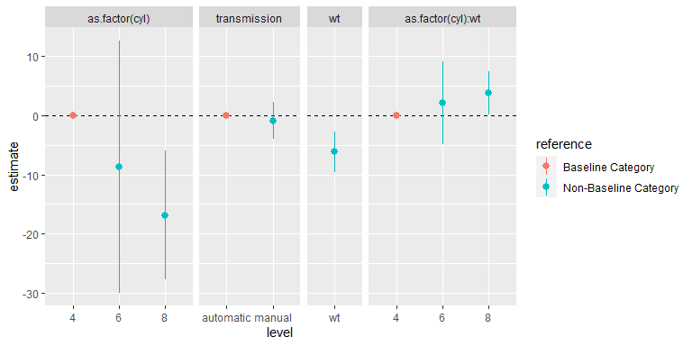
#> 10 as.factor(cyl)8:wt    3.84     0.192      7.50 as.fact~ 8     inter~ Non-Base~

The expanded data frame from tidy_categorical() of parameter estimates can be particularly useful for creating coefficient plots, allowing:

• grouping terms from the same categorical variable from the additional columns.
• inclusion of reference categories in a coefficient plot from the additional rows, allowing the reader to better grasp the meaning of the parameter estimates in each categorical variable.

For example:

library(forcats)
library(ggplot2)
library(ggforce)

d1 %>%
  slice(-1) %>%
  mutate(variable = fct_inorder(variable)) %>%
  ggplot(mapping = aes(x = level, y = estimate, colour = reference,
                       ymin = conf.low, ymax = conf.high)) +
  facet_row(facets = "variable", scales = "free_x", space = "free") +
  geom_hline(yintercept = 0, linetype = "dashed") +
  geom_pointrange()