Overview of the wcde package
Guy J. Abel, Samir K.C., Michaela Potancokova, Claudia Reiter, Andrea Tamburini and Dilek Yildiz
Source:vignettes/wcde.Rmd
wcde.RmdThe wcde package allows for R users to easily download
data from the Wittgenstein Centre
for Demography and Human Capital Data Explorer as well as containing
a number of helpful functions for working with education specific
demographic data.
Installation
You can install the released version of wcde from CRAN with:
install.packages("wcde")Install the developmental version with:
library(devtools)
install_github("guyabel/wcde", ref = "main")
Getting data into R
The get_wcde() function can be used to download data
from the Wittgenstein Centre Human Capital Data Explorer. It requires
three user inputs
-
indicator: a short code for the indicator of interest -
scenario: a number referring to a SSP narrative, by default 2 is used (for SSP2) -
country_code(orcountry_name): corresponding to the country of interest
library(wcde)
# download education specific tfr data
get_wcde(indicator = "etfr",
         country_name = c("Brazil", "Albania"))
#> # A tibble: 192 × 6
#>    scenario name    country_code education          period     etfr
#>       <dbl> <chr>          <dbl> <chr>              <chr>     <dbl>
#>  1        2 Brazil            76 No Education       2020-2025  2.24
#>  2        2 Albania            8 No Education       2020-2025  2.31
#>  3        2 Brazil            76 Incomplete Primary 2020-2025  2.24
#>  4        2 Albania            8 Incomplete Primary 2020-2025  2.51
#>  5        2 Brazil            76 Primary            2020-2025  2.24
#>  6        2 Albania            8 Primary            2020-2025  2.17
#>  7        2 Brazil            76 Lower Secondary    2020-2025  1.78
#>  8        2 Albania            8 Lower Secondary    2020-2025  1.88
#>  9        2 Brazil            76 Upper Secondary    2020-2025  1.35
#> 10        2 Albania            8 Upper Secondary    2020-2025  1.61
#> # ℹ 182 more rows

# download education specific survivorship rates
get_wcde(indicator = "eassr",
         country_name = c("Niger", "Korea"))
#> # A tibble: 8,448 × 8
#>    scenario name              country_code age    sex   education   period eassr
#>       <dbl> <chr>                    <dbl> <chr>  <chr> <chr>       <chr>  <dbl>
#>  1        2 Niger                      562 15--19 Male  No Educati… 2020-… 0.986
#>  2        2 Republic of Korea          410 15--19 Male  No Educati… 2020-… 0.999
#>  3        2 Niger                      562 15--19 Male  Incomplete… 2020-… 0.988
#>  4        2 Republic of Korea          410 15--19 Male  Incomplete… 2020-… 0.999
#>  5        2 Niger                      562 15--19 Male  Primary     2020-… 0.989
#>  6        2 Republic of Korea          410 15--19 Male  Primary     2020-… 0.999
#>  7        2 Niger                      562 15--19 Male  Lower Seco… 2020-… 0.992
#>  8        2 Republic of Korea          410 15--19 Male  Lower Seco… 2020-… 0.999
#>  9        2 Niger                      562 15--19 Male  Upper Seco… 2020-… 0.992
#> 10        2 Republic of Korea          410 15--19 Male  Upper Seco… 2020-… 0.999
#> # ℹ 8,438 more rows
Indicator codes
The indicator input must match the short code from the indicator
table. The find_indicator() function can be used to look up
short codes (given in the first column) from the
wic_indicators data frame:
find_indicator(x = "tfr")
#> # A tibble: 2 × 6
#>   indicator description          `wcde-v3` `wcde-v2` `wcde-v1` definition_latest
#>   <chr>     <chr>                <chr>     <chr>     <chr>     <chr>
#> 1 etfr      Total Fertility Rat… projecti… projecti… projecti… The average numb…
#> 2 tfr       Total Fertility Rate past-ava… past-ava… past-ava… The average numb…
Temporal coverage
By default, get_wdce() returns data for all years or
available periods or years. The filter() function in dplyr can
be used to filter data for specific years or periods, for example:
library(tidyverse)
get_wcde(indicator = "e0",
         country_name = c("Japan", "Australia")) %>%
  filter(period == "2015-2020")
#> # A tibble: 4 × 6
#>   scenario name      country_code sex    period       e0
#>      <dbl> <chr>            <dbl> <chr>  <chr>     <dbl>
#> 1        2 Japan              392 Male   2015-2020  81.1
#> 2        2 Australia           36 Male   2015-2020  81.1
#> 3        2 Japan              392 Female 2015-2020  87.3
#> 4        2 Australia           36 Female 2015-2020  85.1

get_wcde(indicator = "sexratio",
         country_name = c("China", "South Korea")) %>%
  filter(year == 2020)
#> # A tibble: 44 × 6
#>    scenario name              country_code age     year sexratio
#>       <dbl> <chr>                    <dbl> <chr>  <dbl>    <dbl>
#>  1        2 China                      156 All     2020     1.05
#>  2        2 Republic of Korea          410 All     2020     1
#>  3        2 China                      156 0--4    2020     1.14
#>  4        2 Republic of Korea          410 0--4    2020     1.05
#>  5        2 China                      156 5--9    2020     1.16
#>  6        2 Republic of Korea          410 5--9    2020     1.05
#>  7        2 China                      156 10--14  2020     1.17
#>  8        2 Republic of Korea          410 10--14  2020     1.07
#>  9        2 China                      156 15--19  2020     1.17
#> 10        2 Republic of Korea          410 15--19  2020     1.08
#> # ℹ 34 more rows
Past data is only available for selected indicators. These can be viewed using the version column:
wic_indicators %>%
  filter(`wcde-v3` == "past-available") %>%
  select(1:2)
#> # A tibble: 28 × 2
#>    indicator description
#>    <chr>     <chr>
#>  1 asfr      Age-Specific Fertility Rate
#>  2 assr      Age-Specific Survival Ratio
#>  3 bmys      Mean Years of Schooling by Broad Age
#>  4 bpop      Population Size by Broad Age (000's)
#>  5 bprop     Educational Attainment Distribution by Broad Age
#>  6 cbr       Crude Birth Rate
#>  7 cdr       Crude Death Rate
#>  8 e0        Life Expectancy at Birth
#>  9 epop      Population Size by Education (000's)
#> 10 ggapedu15 Gender Gap in Educational Attainment (15+)
#> # ℹ 18 more rows
The filter() function can also be used to filter
specific indicators to specific age, sex or education groups
Country names and codes
Country names are guessed using the countrycode package.
get_wcde(indicator = "tfr",
         country_name = c("U.A.E", "Espania", "Österreich"))
#> # A tibble: 90 × 5
#>    scenario name                 country_code period      tfr
#>       <dbl> <chr>                       <dbl> <chr>     <dbl>
#>  1        2 United Arab Emirates          784 1950-1955  6.88
#>  2        2 Spain                         724 1950-1955  2.49
#>  3        2 Austria                        40 1950-1955  2.08
#>  4        2 United Arab Emirates          784 1955-1960  6.81
#>  5        2 Spain                         724 1955-1960  2.65
#>  6        2 Austria                        40 1955-1960  2.52
#>  7        2 United Arab Emirates          784 1960-1965  6.65
#>  8        2 Spain                         724 1960-1965  2.82
#>  9        2 Austria                        40 1960-1965  2.78
#> 10        2 United Arab Emirates          784 1965-1970  6.50
#> # ℹ 80 more rows
The get_wcde() functions accepts ISO alpha numeric codes
for countries via the country_code argument:
get_wcde(indicator = "etfr", country_code = c(44, 100))
#> # A tibble: 192 × 6
#>    scenario name     country_code education          period     etfr
#>       <dbl> <chr>           <dbl> <chr>              <chr>     <dbl>
#>  1        2 Bahamas            44 No Education       2020-2025  2.2
#>  2        2 Bulgaria          100 No Education       2020-2025  1.86
#>  3        2 Bahamas            44 Incomplete Primary 2020-2025  2.2
#>  4        2 Bulgaria          100 Incomplete Primary 2020-2025  1.86
#>  5        2 Bahamas            44 Primary            2020-2025  2.2
#>  6        2 Bulgaria          100 Primary            2020-2025  1.86
#>  7        2 Bahamas            44 Lower Secondary    2020-2025  1.74
#>  8        2 Bulgaria          100 Lower Secondary    2020-2025  1.86
#>  9        2 Bahamas            44 Upper Secondary    2020-2025  1.46
#> 10        2 Bulgaria          100 Upper Secondary    2020-2025  1.51
#> # ℹ 182 more rows
A full list of available countries and region aggregates, and their
codes, can be found in the wic_locations data frame.
wic_locations
#> # A tibble: 232 × 8
#>    name               isono continent region dim   `wcde-v3` `wcde-v2` `wcde-v1`
#>    <chr>              <dbl> <chr>     <chr>  <chr> <lgl>     <lgl>     <lgl>
#>  1 World                900 NA        NA     area  TRUE      TRUE      TRUE
#>  2 Africa               903 NA        NA     area  TRUE      TRUE      TRUE
#>  3 Asia                 935 NA        NA     area  TRUE      TRUE      TRUE
#>  4 Europe               908 NA        NA     area  TRUE      TRUE      TRUE
#>  5 Latin America and…   904 NA        NA     area  TRUE      TRUE      TRUE
#>  6 Northern America     905 NA        NA     area  TRUE      TRUE      TRUE
#>  7 Oceania              909 NA        NA     area  TRUE      TRUE      TRUE
#>  8 Afghanistan            4 Asia      South… coun… TRUE      TRUE      TRUE
#>  9 Albania                8 Europe    South… coun… TRUE      TRUE      TRUE
#> 10 Algeria               12 Africa    North… coun… TRUE      TRUE      TRUE
#> # ℹ 222 more rows
Scenarios
By default get_wcde() returns data for Medium (SSP2)
scenario. Results for different SSP scenarios can be returned by passing
a different (or multiple) scenario values to the scenario
argument in get_data().
get_wcde(indicator = "growth",
         country_name = c("India", "China"),
         scenario = c(1:3, 22, 23)) %>%
  filter(period == "2095-2100")
#> # A tibble: 10 × 5
#>    scenario name  country_code period    growth
#>       <dbl> <chr>        <dbl> <chr>      <dbl>
#>  1        1 India          356 2095-2100   -1
#>  2        1 China          156 2095-2100   -1.1
#>  3        2 India          356 2095-2100   -0.5
#>  4        2 China          156 2095-2100   -1
#>  5        3 India          356 2095-2100    0.2
#>  6        3 China          156 2095-2100   -0.4
#>  7       22 India          356 2095-2100   -0.5
#>  8       22 China          156 2095-2100   -1
#>  9       23 India          356 2095-2100   -0.5
#> 10       23 China          156 2095-2100   -1
Set include_scenario_names = TRUE to include a columns
with the full names of the scenarios
get_wcde(indicator = "tfr",
         country_name = c("Kenya", "Nigeria", "Algeria"),
         scenario = 1:3,
         include_scenario_names = TRUE) %>%
  filter(period == "2045-2050")
#> # A tibble: 9 × 7
#>   scenario scenario_name            scenario_abb name  country_code period   tfr
#>      <dbl> <chr>                    <chr>        <chr>        <dbl> <chr>  <dbl>
#> 1        1 Rapid Development (SSP1) SSP1         Kenya          404 2045-…  1.64
#> 2        1 Rapid Development (SSP1) SSP1         Nige…          566 2045-…  2.62
#> 3        1 Rapid Development (SSP1) SSP1         Alge…           12 2045-…  1.53
#> 4        2 Medium (SSP2)            SSP2         Kenya          404 2045-…  2.34
#> 5        2 Medium (SSP2)            SSP2         Nige…          566 2045-…  3.76
#> 6        2 Medium (SSP2)            SSP2         Alge…           12 2045-…  2.06
#> 7        3 Stalled Development (SS… SSP3         Kenya          404 2045-…  3.04
#> 8        3 Stalled Development (SS… SSP3         Nige…          566 2045-…  4.87
#> 9        3 Stalled Development (SS… SSP3         Alge…           12 2045-…  2.68
Additional details of the pathways for each scenario numeric code can
be found in the wic_scenarios object. Further background
and links to the corresponding literature are provided in the Data
Explorer
wic_scenarios
#> # A tibble: 9 × 6
#>   scenario_name              scenario scenario_abb `wcde-v3` `wcde-v2` `wcde-v1`
#>   <chr>                         <dbl> <chr>        <lgl>     <lgl>     <lgl>
#> 1 Rapid Development (SSP1)          1 SSP1         TRUE      TRUE      TRUE
#> 2 Medium (SSP2)                     2 SSP2         TRUE      TRUE      TRUE
#> 3 Stalled Development (SSP3)        3 SSP3         TRUE      TRUE      TRUE
#> 4 Inequality (SSP4)                 4 SSP4         TRUE      FALSE     TRUE
#> 5 Conventional Development …        5 SSP5         TRUE      FALSE     TRUE
#> 6 Medium - Zero Migration (…       22 SSP2-ZM      TRUE      TRUE      FALSE
#> 7 Medium - Double Migration…       23 SSP2-DM      TRUE      TRUE      FALSE
#> 8 Medium - Constant Enrolme…       20 SSP2-CER     FALSE     FALSE     TRUE
#> 9 Medium - Fast Track Educa…       21 SSP2-FT      FALSE     FALSE     TRUE
All countries data
Data for all countries can be obtained by not setting
country_name or country_code
get_wcde(indicator = "mage")
#> # A tibble: 6,858 × 5
#>    scenario name                     country_code  year  mage
#>       <dbl> <chr>                           <dbl> <dbl> <dbl>
#>  1        2 Bulgaria                          100  1950  26.9
#>  2        2 Myanmar                           104  1950  21.8
#>  3        2 Burundi                           108  1950  19.5
#>  4        2 Belarus                           112  1950  26.6
#>  5        2 Cambodia                          116  1950  18.6
#>  6        2 Algeria                            12  1950  19.5
#>  7        2 Cameroon                          120  1950  20.4
#>  8        2 Canada                            124  1950  27.7
#>  9        2 Cape Verde                        132  1950  17.9
#> 10        2 Central African Republic          140  1950  22.4
#> # ℹ 6,848 more rows
Multiple indicators
The get_wdce() function needs to be called multiple
times to download multiple indicators. This can be done using the
map() function in purrr
mi <- tibble(ind = c("odr", "nirate", "ggapedu25")) %>%
  mutate(d = map(.x = ind, .f = ~get_wcde(indicator = .x)))
mi
#> # A tibble: 3 × 2
#>   ind       d
#>   <chr>     <list>
#> 1 odr       <tibble [6,858 × 5]>
#> 2 nirate    <tibble [6,630 × 5]>
#> 3 ggapedu25 <tibble [52,776 × 6]>

mi %>%
  filter(ind == "odr") %>%
  select(-ind) %>%
  unnest(cols = d)
#> # A tibble: 6,858 × 5
#>    scenario name                     country_code  year   odr
#>       <dbl> <chr>                           <dbl> <dbl> <dbl>
#>  1        2 Bulgaria                          100  1950  0.1
#>  2        2 Myanmar                           104  1950  0.05
#>  3        2 Burundi                           108  1950  0.06
#>  4        2 Belarus                           112  1950  0.13
#>  5        2 Cambodia                          116  1950  0.05
#>  6        2 Algeria                            12  1950  0.06
#>  7        2 Cameroon                          120  1950  0.06
#>  8        2 Canada                            124  1950  0.12
#>  9        2 Cape Verde                        132  1950  0.07
#> 10        2 Central African Republic          140  1950  0.09
#> # ℹ 6,848 more rows

mi %>%
  filter(ind == "nirate") %>%
  select(-ind) %>%
  unnest(cols = d)
#> # A tibble: 6,630 × 5
#>    scenario name                     country_code period    nirate
#>       <dbl> <chr>                           <dbl> <chr>      <dbl>
#>  1        2 Bulgaria                          100 1950-1955   11
#>  2        2 Myanmar                           104 1950-1955   19.8
#>  3        2 Burundi                           108 1950-1955   27.9
#>  4        2 Belarus                           112 1950-1955    9.9
#>  5        2 Cambodia                          116 1950-1955   25.2
#>  6        2 Algeria                            12 1950-1955   29.1
#>  7        2 Cameroon                          120 1950-1955   16.2
#>  8        2 Canada                            124 1950-1955   20
#>  9        2 Cape Verde                        132 1950-1955   27.4
#> 10        2 Central African Republic          140 1950-1955   15.1
#> # ℹ 6,620 more rows

mi %>%
  filter(ind == "ggapedu25") %>%
  select(-ind) %>%
  unnest(cols = d)
#> # A tibble: 52,776 × 6
#>    scenario name                     country_code  year education    ggapedu25
#>       <dbl> <chr>                           <dbl> <dbl> <chr>            <dbl>
#>  1        2 Bulgaria                          100  1950 No Education     -17.8
#>  2        2 Myanmar                           104  1950 No Education     -19.3
#>  3        2 Burundi                           108  1950 No Education     -22.9
#>  4        2 Belarus                           112  1950 No Education     -19.8
#>  5        2 Cambodia                          116  1950 No Education     -27.3
#>  6        2 Algeria                            12  1950 No Education      -1.2
#>  7        2 Cameroon                          120  1950 No Education     -19
#>  8        2 Canada                            124  1950 No Education       0
#>  9        2 Cape Verde                        132  1950 No Education     -23.7
#> 10        2 Central African Republic          140  1950 No Education     -20.2
#> # ℹ 52,766 more rows
Previous versions
Previous versions of projections from the Wittgenstein Centre for
Demography are available using the version argument in
get_wcde(). Set version to "wcde-v1"
or "wcde-v2"
or "wcde-v3"
(the default since 2024).
get_wcde(indicator = "etfr",
         country_name = c("Brazil", "Albania"),
         version = "wcde-v2")
#> # A tibble: 204 × 6
#>    scenario name    country_code education          period     etfr
#>       <dbl> <chr>          <dbl> <chr>              <chr>     <dbl>
#>  1        2 Brazil            76 No Education       2015-2020  2.47
#>  2        2 Albania            8 No Education       2015-2020  1.88
#>  3        2 Brazil            76 Incomplete Primary 2015-2020  2.47
#>  4        2 Albania            8 Incomplete Primary 2015-2020  1.88
#>  5        2 Brazil            76 Primary            2015-2020  2.47
#>  6        2 Albania            8 Primary            2015-2020  1.88
#>  7        2 Brazil            76 Lower Secondary    2015-2020  1.89
#>  8        2 Albania            8 Lower Secondary    2015-2020  1.9
#>  9        2 Brazil            76 Upper Secondary    2015-2020  1.37
#> 10        2 Albania            8 Upper Secondary    2015-2020  1.57
#> # ℹ 194 more rows
Note, not all indicators and scenarios are available in all versions
- see the the wic_indicators and wic_scenarios
objects for further details or see above.
Server
If you have trouble with connecting to the IIASA server you can try
alternative hosts using the server option in
get_wcde(), which can be set to "iiasa"
(default) "github" and "1&1".
get_wcde(indicator = "etfr",
         country_name = c("Brazil", "Albania"),
         server = "github")
#> # A tibble: 192 × 6
#>    scenario name    country_code education          period     etfr
#>       <dbl> <chr>          <dbl> <chr>              <chr>     <dbl>
#>  1        2 Brazil            76 No Education       2020-2025  2.24
#>  2        2 Albania            8 No Education       2020-2025  2.31
#>  3        2 Brazil            76 Incomplete Primary 2020-2025  2.24
#>  4        2 Albania            8 Incomplete Primary 2020-2025  2.51
#>  5        2 Brazil            76 Primary            2020-2025  2.24
#>  6        2 Albania            8 Primary            2020-2025  2.17
#>  7        2 Brazil            76 Lower Secondary    2020-2025  1.78
#>  8        2 Albania            8 Lower Secondary    2020-2025  1.88
#>  9        2 Brazil            76 Upper Secondary    2020-2025  1.35
#> 10        2 Albania            8 Upper Secondary    2020-2025  1.61
#> # ℹ 182 more rows
You may also set server = "search-available" to search
through the three possible data location to download the data wherever
it is available.
Working with population data
Population data for a range of age-sex-educational attainment
combinations can be obtained by setting indicator = "pop"
in get_wcde() and specifying a pop_age,
pop_sex and pop_edu arguments. By default each
of the three population breakdown arguments are set to “total”
get_wcde(indicator = "pop", country_name = "India")
#> # A tibble: 31 × 5
#>    scenario name  country_code  year     pop
#>       <dbl> <chr>        <dbl> <dbl>   <dbl>
#>  1        2 India          356  1950 353104.
#>  2        2 India          356  1955 394095
#>  3        2 India          356  1960 440828.
#>  4        2 India          356  1965 494677.
#>  5        2 India          356  1970 551306.
#>  6        2 India          356  1975 616603.
#>  7        2 India          356  1980 688875.
#>  8        2 India          356  1985 771520.
#>  9        2 India          356  1990 861205.
#> 10        2 India          356  1995 954786.
#> # ℹ 21 more rows
The pop_age argument can be set to all to
get population data broken down in five-year age groups. The
pop_sex argument can be set to both to get
population data broken down into female and male groups. The
pop_edu argument can be set to four,
six or eight to get population data broken
down into education categorizations with different levels of detail.
get_wcde(indicator = "pop", country_code = 900, pop_edu = "four")
#> # A tibble: 155 × 6
#>    scenario name  country_code  year education          pop
#>       <dbl> <fct>        <dbl> <dbl> <fct>            <dbl>
#>  1        2 World          900  1950 Under 15       857662.
#>  2        2 World          900  1950 No Education   779147.
#>  3        2 World          900  1950 Primary        495037.
#>  4        2 World          900  1950 Secondary      320938.
#>  5        2 World          900  1950 Post Secondary  24890.
#>  6        2 World          900  1955 Under 15       971774.
#>  7        2 World          900  1955 No Education   779160.
#>  8        2 World          900  1955 Primary        548060
#>  9        2 World          900  1955 Secondary      384565.
#> 10        2 World          900  1955 Post Secondary  35093.
#> # ℹ 145 more rows
The population breakdown arguments can be used in combination to provide further breakdowns, for example sex and education specific population totals
get_wcde(indicator = "pop", country_code = 900, pop_edu = "six", pop_sex = "both")
#> # A tibble: 434 × 7
#>    scenario name  country_code  year sex    education              pop
#>       <dbl> <fct>        <dbl> <dbl> <fct>  <fct>                <dbl>
#>  1        2 World          900  1950 Male   Under 15           438532.
#>  2        2 World          900  1950 Male   No Education       333362
#>  3        2 World          900  1950 Male   Incomplete Primary 109944.
#>  4        2 World          900  1950 Male   Primary            167428.
#>  5        2 World          900  1950 Male   Lower Secondary    102241.
#>  6        2 World          900  1950 Male   Upper Secondary     66705.
#>  7        2 World          900  1950 Male   Post Secondary      16416.
#>  8        2 World          900  1950 Female Under 15           419131.
#>  9        2 World          900  1950 Female No Education       445785.
#> 10        2 World          900  1950 Female Incomplete Primary  72736.
#> # ℹ 424 more rows
The full age-sex-education specific data can also be obtained by
setting indicator = "epop" in get_wcde().
Population pyramids
Create population pyramids by setting male population values to negative equivalent to allow for divergent columns from the y axis.
w <- get_wcde(indicator = "pop", country_code = 900,
              pop_age = "all", pop_sex = "both", pop_edu = "four",
              version = "wcde-v3")
w
#> # A tibble: 4,650 × 8
#>    scenario name  country_code  year age    sex    education          pop
#>       <dbl> <fct>        <dbl> <dbl> <fct>  <fct>  <fct>            <dbl>
#>  1        2 World          900  1950 0--4   Male   Under 15       170451.
#>  2        2 World          900  1950 0--4   Female Under 15       163206.
#>  3        2 World          900  1950 5--9   Male   Under 15       136460.
#>  4        2 World          900  1950 5--9   Female Under 15       130304.
#>  5        2 World          900  1950 10--14 Male   Under 15       131621.
#>  6        2 World          900  1950 10--14 Female Under 15       125620
#>  7        2 World          900  1950 15--19 Male   No Education    33724.
#>  8        2 World          900  1950 15--19 Male   Primary         49895
#>  9        2 World          900  1950 15--19 Male   Secondary       35984.
#> 10        2 World          900  1950 15--19 Male   Post Secondary    312.
#> # ℹ 4,640 more rows

w <- w %>%
  mutate(pop_pm = ifelse(test = sex == "Male", yes = -pop, no = pop),
         pop_pm = pop_pm/1e3)
w
#> # A tibble: 4,650 × 9
#>    scenario name  country_code  year age    sex    education        pop   pop_pm
#>       <dbl> <fct>        <dbl> <dbl> <fct>  <fct>  <fct>          <dbl>    <dbl>
#>  1        2 World          900  1950 0--4   Male   Under 15      1.70e5 -170.
#>  2        2 World          900  1950 0--4   Female Under 15      1.63e5  163.
#>  3        2 World          900  1950 5--9   Male   Under 15      1.36e5 -136.
#>  4        2 World          900  1950 5--9   Female Under 15      1.30e5  130.
#>  5        2 World          900  1950 10--14 Male   Under 15      1.32e5 -132.
#>  6        2 World          900  1950 10--14 Female Under 15      1.26e5  126.
#>  7        2 World          900  1950 15--19 Male   No Education  3.37e4  -33.7
#>  8        2 World          900  1950 15--19 Male   Primary       4.99e4  -49.9
#>  9        2 World          900  1950 15--19 Male   Secondary     3.60e4  -36.0
#> 10        2 World          900  1950 15--19 Male   Post Seconda… 3.12e2   -0.312
#> # ℹ 4,640 more rows
Standard plot
Use standard ggplot code to create population pyramid with
-
scale_x_symmetric()from thelemonpackage to allow for equal male and female x-axis - fill colours set to the
wic_col4object in the wcde package which contains the names of the colours used in the Wittgenstein Centre Human Capital Data Explorer Data Explorer.
Note wic_col6 and wic_col8 objects also
exist for equivalent plots of population data objects with corresponding
numbers of categories of education.
library(lemon)

w %>%
  filter(year == 2020) %>%
  ggplot(mapping = aes(x = pop_pm, y = age, fill = fct_rev(education))) +
  geom_col() +
  geom_vline(xintercept = 0, colour = "black") +
  scale_x_symmetric(labels = abs) +
  scale_fill_manual(values = wic_col4, name = "Education") +
  labs(x = "Population (millions)", y = "Age") +
  theme_bw()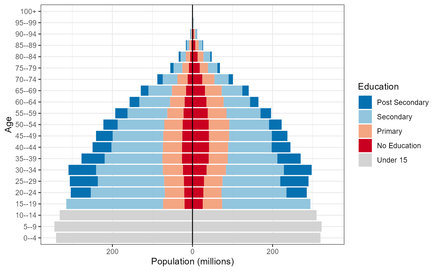
Sex label position
Add male and female labels on the x-axis by
- Creating a facet plot with the strips on the bottom with transparent backgrounds and no space between.
- Set the x axis to have zero expansion beyond the values in the data allowing the two sides of the pyramids to meet.
- Add a
geom_blank()to allow for equal x-axis and additional space at the end of largest columns.
w <- w %>%
  mutate(pop_max = ifelse(sex == "Male", -max(pop/1e3), max(pop/1e3)))

w %>%
  filter(year == 2020) %>%
  ggplot(mapping = aes(x = pop_pm, y = age, fill = fct_rev(education))) +
  geom_col() +
  geom_vline(xintercept = 0, colour = "black") +
  scale_x_continuous(labels = abs, expand = c(0, 0)) +
  scale_fill_manual(values = wic_col4, name = "Education") +
  labs(x = "Population (millions)", y = "Age") +
  facet_wrap(facets = "sex", scales = "free_x", strip.position = "bottom") +
  geom_blank(mapping = aes(x = pop_max * 1.1)) +
  theme(panel.spacing.x = unit(0, "pt"),
        strip.placement = "outside",
        strip.background = element_rect(fill = "transparent"),
        strip.text.x = element_text(margin = margin( b = 0, t = 0)))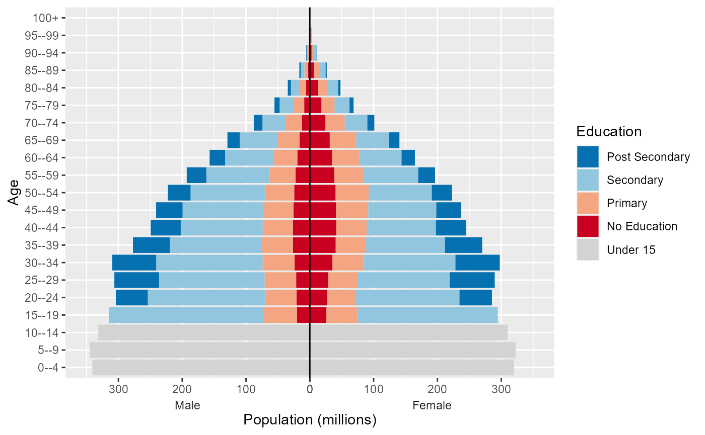
Animate
Animate the pyramid through the past data and projection periods
using the transition_time() function in the gganimate
package
library(gganimate)

ggplot(data = w,
       mapping = aes(x = pop_pm, y = age, fill = fct_rev(education))) +
  geom_col() +
  geom_vline(xintercept = 0, colour = "black") +
  scale_x_continuous(labels = abs, expand = c(0, 0)) +
  scale_fill_manual(values = wic_col4, name = "Education") +
  facet_wrap(facets = "sex", scales = "free_x", strip.position = "bottom") +
  geom_blank(mapping = aes(x = pop_max * 1.1)) +
  theme(panel.spacing.x = unit(0, "pt"),
        strip.placement = "outside",
        strip.background = element_rect(fill = "transparent"),
        strip.text.x = element_text(margin = margin(b = 0, t = 0))) +
  transition_time(time = year) +
  labs(x = "Population (millions)", y = "Age",
       title = 'SSP2 World Population {round(frame_time)}')