The fanplot package for R

Visualising Time Series Model Results

The fanplot package is designed to help display uncertainty in estimates from time series models. To illustrate, the packages th.mcmc data frame object contains posterior density distributions of the estimated volatility of daily returns \(y_t\) from the Pound/Dollar exchange rate from 02/10/1981 to 28/6/1985. These distributions are from a MCMC simulation from a stochastic volatility model given in Meyer and Yu (2002) where it assumed;

\[ y_t | \theta_t = \exp\left(\frac{1}{2}\theta_t\right)u_t \qquad u_t \sim N(0, 1) \qquad t=1,\ldots,n. \]

The latent volatilities \(\theta_t\), which are unknown states in a state-space model terminology, are assumed to follow a Markovian transition over time given by the state equations:

\[ \theta_t | \theta_{t-1}, \mu, \phi, \tau^2 = \mu + \phi \log \sigma^2_{t-1} + v_t \qquad v_t \sim N(0, \tau^2) \qquad t=1,\ldots,n \]

with \(\theta_0 \sim N(\mu, \tau^2)\).

The th.mcmc object consists of (1000) rows corresponding to MCMC simulations and (945) columns corresponding to each \(t\). A fan chart of the evolution of the distribution of \(\theta_t\) can be visualised using the fanplot package via,

library(fanplot)
# empty plot
plot(NULL, main="Percentiles", xlim = c(1, 965), ylim = c(-2.5, 1.5))

# add fan
fan(data = th.mcmc)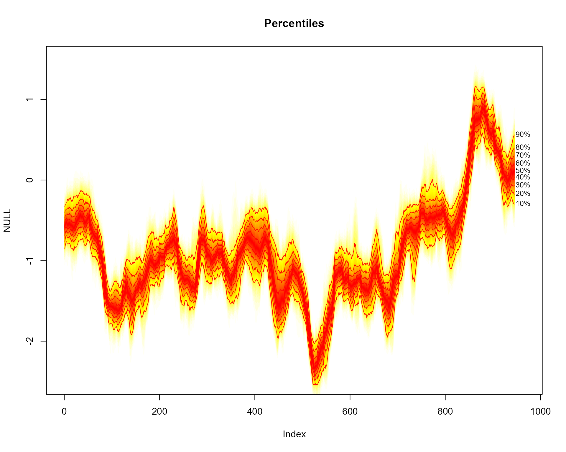

The fan() function calculates the values of 100 equally spaced percentiles of each future distribution when the default data.type = "simulations" is set. This allows 50 fans to be plotted from the heat.colours colour palette, providing a fine level of shading. In addition, lines and labels are provided along each decile.

Prediction Intervals

When argument type = "interval" is set, the probs argument corresponds to prediction intervals. Consequently, the fan chart comprises of 3 different shades, running from the darkest shade for the 50th prediction interval to the lightest for the 95th prediction interval.

# empty plot
plot(NULL, main="Prediction Intervals", xlim = c(-20, 965), ylim = c(-2.5, 1.5))

# add fan
fan(data = th.mcmc, type = "interval", llab=TRUE, rcex=0.6)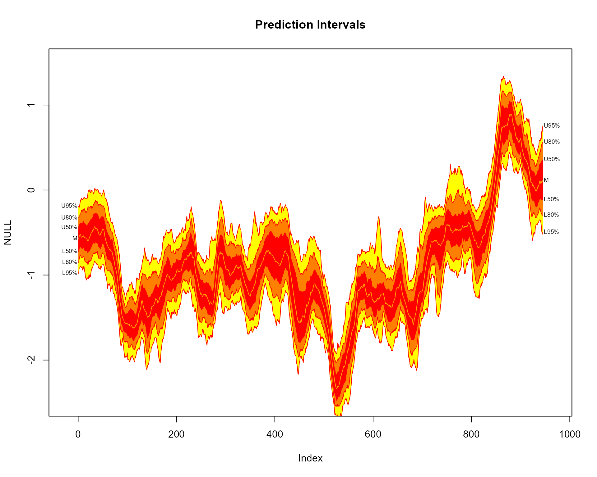

Contour lines are overlayed for the upper and lower bounds of each prediction intervals, as set using the ln command. A further line is plotted along the median of \(\theta_t\), which is controlled by the med.ln argument (set to TRUE by default when type="interval"). The default labels on the right hand side correspond to the upper and lower bounds of each plotted line. The left labels are added by setting llab = TRUE. Note, some extra room is created for the labels by setting the xlim = c(-20, 965) argument of plotting area to a wider range than the original data (945 observations). The text size of the right labels are controlled using the rcex argument. The left labels, by default, take the same text size as rcex although they can be separately controlled using the lcex argument.

Alternative Colours

Alternative colour schemes to the default heat.colors, can be obtained by supplying a colorRampPalette to the fan.col argument. For example, a new palette running from blue to white, via grey can be passed using;

# empty plot
plot(NULL, xlim = c(-20, 965), ylim = c(-2.5, 1.5),  main="Alternative Colour Scheme")

# add fan
fan(data = th.mcmc, rlab=seq(20,80,15), llab=c(10,50,90), fan.col=colorRampPalette(c("royalblue", "grey", "white")))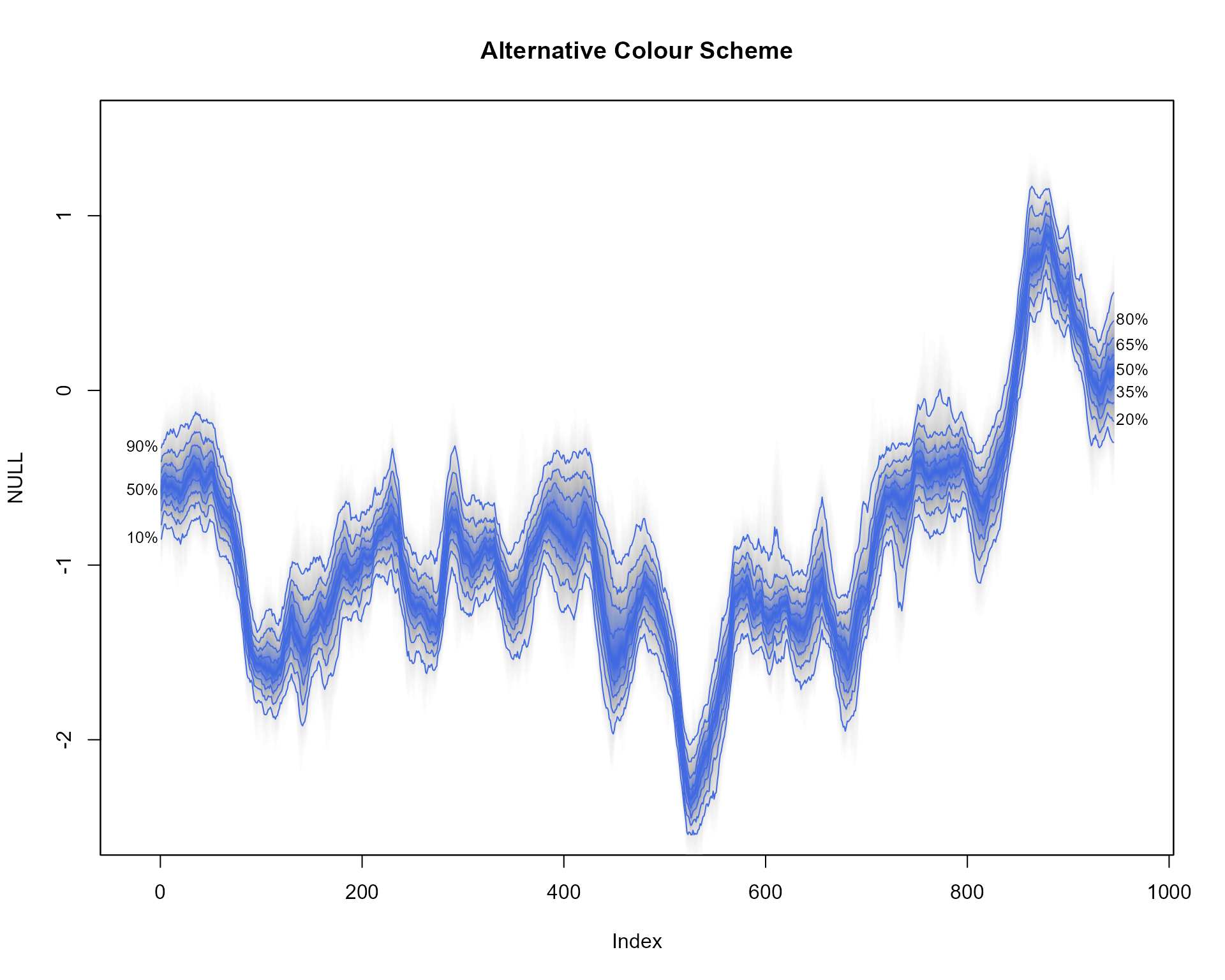

Alternative labels are specified using the rlab and llab arguments.

Spaghetti Plots

Spaghetti plots can be used to represent uncertainty shown by a range of possible future trajectories or past estimates. For example using the th.mcmc object, 20 random sets of \(\theta_t\) can be plotted when setting the argument style = "spaghetti";

# empty plot
plot(NULL, main="Spaghetti Plot", xlim = c(-20, 965), ylim = range(th.mcmc))

# transparent fan with visible lines
fan(th.mcmc, ln=c(5, 50, 95), llab=TRUE, alpha=0, ln.col="orange")

# spaghetti lines
fan(th.mcmc, style="spaghetti", n.spag=20)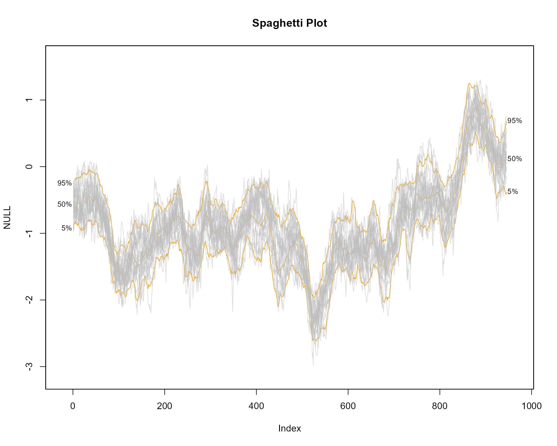

The spaghetti lines are superimposed on a fan chart in order to illustrate some underlying probabilities. The initial fan chart is completely transparent from setting the transparency argument alpha to 0. In order for the percentile lines to be visible a non-transparent colour is used for the ln.col argument.

Forecast Fans

The fanplot package can also be used to illustrate probabilistic forecasts. For example, using the auto.arima function in the forecast package a model for the time series for net migration to the United Kingdom (contained in the ips data frame of the fanplot package) can be fitted.

#create time series
net <- ts(ips$net, start = 1975)

#fit model
library(forecast)
m <- auto.arima(net)
m

## Series: net 
## ARIMA(1,1,2) with drift 
## 
## Coefficients:
##           ar1      ma1      ma2   drift
##       -0.2301  -0.0851  -0.6734  6.7625
## s.e.   0.3664   0.3571   0.1898  1.3961
## 
## sigma^2 = 1343:  log likelihood = -184.28
## AIC=378.56   AICc=380.5   BIC=386.62

We may then simulate 1000 values from the selected model using the simulate.Arima function, and plot the results.

mm <- matrix(NA, nrow=1000, ncol=5)
for(i in 1:1000)
  mm[i,] <- simulate(m, nsim=5)

# empty plot
plot(net, main="UK Net Migration", xlim=c(1975,2020), ylim=c(-100,300))

# add fan
fan(mm, start=2013)

Users might want to connect the fan with the past data. This can be achieved by providing the last value to the anchor argument. More shades for the fan are added to the plot (over the default 3 used for a interval fans) by supplying a sequence to the probs argument. Alternative contour lines (from the default median, 50th, 80th and 95th percentiles for interval fans) are added using the ln argument.

# empty plot
plot(net, main="UK Net Migration", xlim=c(1975,2020), ylim=c(-100,300))

# add fan
fan(mm, start=2013, anchor=net[time(net)==2012], type="interval", probs=seq(5, 95, 5), ln=c(50, 80))

Guy J. Abel

Visualising Time Series Model Results

Prediction Intervals

Alternative Colours

Spaghetti Plots

Forecast Fans